Housing Pressure, Youth Unemployment, and Fertility Responses to Economic Downturns in Europe

Abstract

Europe’s renewed fertility decline has intensified concern about whether adverse economic conditions delay or suppress family formation, yet average macroeconomic effects may conceal the household constraints through which shocks operate. This study distinguishes the direct effects of housing-cost pressure and youth unemployment from their moderating roles in the relationship between economic downturns and the total fertility rate (TFR). The principal analysis uses a common sample of 565 country-year observations from 36 European countries during 2005–2024. Real GDP-per-capita growth is decomposed into expansions and downturns. The main country- and year-fixed-effects specifications use two-year-lagged predictors and country-clustered standard errors. No general direct effect of downturns is detected. In the preferred joint model, the downturn × housing-pressure interaction is negative and statistically significant (b = −0.0035, SE = 0.0013, p = .012), whereas the downturn × youth-unemployment interaction is small and not statistically significant (b = 0.0006, SE = 0.0019, p = .739). Youth unemployment has a negative direct association with fertility when entered without aggregate unemployment (b = −0.0632, p = .013), but youth and aggregate unemployment are highly correlated and cannot be cleanly separated when entered together. The housing interaction remains significant with two-way-clustered and Driscoll–Kraay standard errors and in several robustness models, but not under all lag and country-trend specifications. Its substantive magnitude is modest: a five-percentage-point downturn at one standard deviation above mean housing pressure is associated with an estimated TFR change of −0.0086 (95% CI: −0.0562, 0.0390). The findings therefore support a cautious conditional interpretation: housing pressure is associated with a more negative downturn–fertility slope, while youth unemployment is more consistently related to fertility directly than as a moderator.

1 Introduction

Europe is entering a period in which very low fertility is no longer confined to a small group of countries or to a temporary phase of postponement. In 2024, the total fertility rate (TFR) of the European Union fell to 1.34 births per woman, the lowest value recorded for the EU series since 2001, while the number of births declined to 3.55 million (Eurostat, 2026). This decline is demographically consequential because it interacts with population ageing, smaller cohorts entering the labour market, regional depopulation, and widening gaps between desired and realised family size. Recent European assessments consequently emphasise that no single mechanism can explain low fertility and that the relative importance of economic security, housing, gender relations, partnership formation, and family policy varies across countries and social groups (Bignami et al., 2024; OECD, 2024).

A central empirical question is whether deteriorating macroeconomic conditions reduce fertility uniformly, or whether their demographic consequences depend on the constraints already facing prospective parents. Classical economic accounts connect fertility to income, opportunity costs, and investments in child quality (Becker, 1960, 1991; Becker & Lewis, 1973), whereas Easterlin’s framework stresses relative economic position and cohort opportunity (Easterlin, 1975). Research on economic crises and unemployment has shown that fertility commonly responds procyclically, but the magnitude, timing, and persistence of the response differ across countries, educational groups, and welfare regimes (Adsera, 2004, 2005, 2011; Comolli, 2017; Goldstein et al., 2009; Schneider, 2015; Sobotka et al., 2011). These differences caution against treating aggregate GDP growth as a sufficient description of the economic environment in which family decisions are made.

The contemporary literature increasingly interprets fertility decisions as contingent on whether young adults can reach socially expected prerequisites for parenthood. Employment uncertainty, weak income prospects, and the risk of downward mobility can encourage postponement, especially around first births (Alderotti et al., 2021; Kreyenfeld, 2010; Matysiak & Vignoli, 2024). Recent evidence also suggests that the income prerequisites of parenthood have become more demanding: income has grown more strongly associated with entry into parenthood, even when the perceived uncertainty itself does not show a consistently intensifying effect (van Wijk & Billari, 2024). Youth unemployment is therefore relevant not merely as a cyclical indicator, but as a marker of difficulty in establishing the employment trajectories on which residential independence and family formation frequently depend.

Housing is the second prerequisite. Leaving the parental home, establishing a partnership, and having a child are closely connected to housing tenure, space, stability, and affordability (Kulu & Steele, 2013; Mulder, 2006; Mulder & Billari, 2010). High housing costs can postpone household formation among renters and potential first-time buyers, while owners may experience a positive wealth channel when house prices rise (Dettling & Kearney, 2014). New evidence from the Netherlands shows that rising prices can widen fertility differences between housing-market insiders and outsiders, with lower conception risks among renters in expensive areas and positive equity effects among established owners (van Wijk, 2024; van Wijk & Feijten, 2025). Housing pressure may thus operate both as a direct constraint and as a moderator that changes how strongly an economic downturn translates into fertility change.

Family-policy institutions may buffer these pressures, but their effects are neither automatic nor uniform. Paid leave, childcare, and financial supports can reduce the opportunity and direct costs of children, particularly when they facilitate the combination of employment and family life (Gauthier, 2007; Kalwij, 2010; Neyer & Andersson, 2008; OECD, 2024). By contrast, pronatalist cash or housing-linked subsidies may produce heterogeneous, temporary, or timing-specific responses. Hungary’s Family Housing Allowance (CSOK) links housing grants and subsidised finance to the number of existing or promised children. Russia’s Maternity Capital programme, initially targeted at second and subsequent births, permits eligible families to improve housing conditions, finance children’s education or childcare, or contribute to the mother’s pension. Evidence from Poland’s Family 500+ programme, CSOK and related Hungarian instruments, and Russia’s maternity-capital schemes suggests that effects depend on eligibility, parity, targeting, and institutional credibility; they may accelerate births, or affect selected parity transitions without ensuring a sustained aggregate fertility recovery (Bokun, 2024; Proshin, 2023; Sági & Lentner, 2022; Slonimczyk & Yurko, 2014; Vakulenko et al., 2023).

This study asks three related questions. First, do European fertility rates respond differently to economic expansions and downturns? Second, are housing pressure and youth unemployment directly associated with fertility after country and year fixed effects are taken into account? Third, do these factors condition the fertility response to expansions and downturns? The distinction between direct and moderating roles is explicit. Housing pressure and youth unemployment enter first as direct predictors, to be subsequently interacting separately and jointly with the two components of GDP-per-capita growth. Aggregate unemployment is analysed as an alternative labour-market indicator, rather than being treated only as a control alongside a highly correlated youth series.

The study contributes in four ways. It decomposes macroeconomic growth into expansions and downturns; makes the direct-versus-moderating distinction operational for both housing pressure and youth unemployment; uses two-year lags as the principal timing structure; and subjects the results to fixed-effects, random-effects, correlated-random-effects, serial-dependence, non-stationarity, regional, dynamic, and family-policy sensitivity analyses. Female labour-force participation and female tertiary enrolment are retained as theoretically relevant controls, rather than being presented as separate headline mechanisms. The results show no broad direct downturn effect. Housing pressure is associated with a more negative downturn–fertility slope in the principal two-year-lag models, but the estimated magnitude is small and sensitive to some timing and trend specifications. Youth unemployment is negatively associated with fertility directly, but does not consistently moderate downturn effects.

2 Theoretical Framework and Hypotheses

2.1 Economic cycles, uncertainty, and fertility

Economic models predict that fertility may respond to the balance between household resources and the opportunity costs of time. A downturn can reduce current and expected income, weaken employment security, and raise uncertainty, which may encourage postponement. At the same time, lower employment may reduce the opportunity cost of childbearing for some groups. The aggregate sign is therefore theoretically ambiguous and empirically dependent on labour-market institutions, gender arrangements, and the duration of the shock (Adsera, 2004; Andersson, 2000; Currie & Schwandt, 2014).

The study does not assume that expansions and contractions have equal and opposite demographic effects. Positive and negative GDP-per-capita growth are represented by separate non-negative variables. The first hypothesis is deliberately modest: economic downturns are expected to have a non-positive association with fertility, but the analysis allows the average effect to be weak or null if institutional and household contexts offset one another.

H1. Larger economic downturns are associated with lower TFR, conditional on country and year fixed effects and socioeconomic controls.

2.2 Housing pressure as a direct constraint and moderator

Housing affects the feasibility and timing of family formation through affordability, residential independence, dwelling size, tenure security, and wealth. The housing-cost overburden rate captures the share of the population whose housing costs exceed the Eurostat threshold relative to disposable income. Unlike a house-price index, it directly represents the burden on household budgets and therefore aligns with the proposed mechanism.

The moderation argument is that a given macroeconomic contraction may be more consequential when housing already absorbs a large portion of disposable resources. In such settings, income loss or heightened uncertainty can more readily interrupt moves, partnership formation, or plans for a child. The interaction between the absolute size of a downturn and standardised housing pressure is therefore the main parameter of interest.

H2a. Higher housing-cost pressure is directly associated with lower TFR.

H2b. Housing pressure makes the association between economic downturns and TFR more negative.

2.3 Youth unemployment as a direct constraint and moderator

Youth unemployment is used as an indicator of labour-market insecurity during the transition to adulthood. The WDI/ILO series covers ages 15–24. This definition is transparent and internationally comparable, but it is lower than the median age at first birth in most contemporary European populations. It is therefore interpreted as a macro-level indicator of early labour-market integration and delayed economic independence, not as a direct measure of unemployment among all prospective parents.

Youth unemployment may lower fertility directly by delaying stable employment, residential independence, and partnership transitions. It may also moderate macroeconomic shocks if downturns are especially consequential where young people already face weak labour-market access. Because aggregate unemployment could be equally or more relevant, the analysis estimates parallel models in which youth and aggregate unemployment enter separately.

H3a. Higher youth unemployment is directly associated with lower TFR.

H3b. Youth unemployment makes the association between economic downturns and TFR more negative.

2.4 Family policies and regional housing regimes

European housing and family regimes differ in the balance between homeownership, social renting, intergenerational support, labour-market protection, and public care. Southern European settings have often been characterised by high homeownership aspirations, limited affordable rental alternatives, late home-leaving, and strong reliance on family support (Castles & Ferrera, 1996; Mulder & Billari, 2010). Recent evidence continues to document marked European differences in leaving-home intentions and housing autonomy. Economic vulnerability has been particularly consequential for young adults in Italy and Spain, while evidence from Catalonia shows that intermediate forms of residential independence often remain tied to parental resources and support (Gil-Solsona, 2023; Luppi et al., 2024; Schwanitz et al., 2021). These features motivate, but do not predetermine, a regional housing test. The empirical analysis therefore estimates whether the downturn × housing interaction is stronger in Southern Europe, and also reports all four regional slopes.

Family-policy controls are introduced in reduced samples to assess whether the main conditional relationships are absorbed by public spending on family and children, formal childcare participation, parental-leave expenditure, childcare expenditure, cash family benefits, or total in-kind family benefits. Each augmented policy model is paired with an otherwise identical baseline estimated on the same observations, preventing sample composition from being mistaken for a policy-control effect.

3 Data and Methods

3.1 Data sources, period, and study sample

The analysis combines annual country-level data from the World Bank World Development Indicators (WDI), Eurostat, and the OECD Social Expenditure Database. The empirical study sample covers 36 European countries during 2005–2024. A one-year-lag complete-case specification contains 598 country-year observations, whereas the principal two-year-lag common sample contains 565 observations. The principal models require complete information on two-year-lagged housing pressure, youth unemployment, GDP per capita, female labour-force participation, and female tertiary enrolment.

Using the same 565 country-year observations for Models M1–M6 ensures that changes in coefficients across specifications reflect model content rather than changes in countries or years. The regional distribution of the principal sample is 98 observations from seven Western European countries, 105 observations from six Eastern European countries, 180 observations from ten Northern European countries, and 182 observations from thirteen Southern European countries. The country-level composition of the principal estimation sample is provided in Table A1 in the Appendix.

The definitions, measurements, and data sources of the variables used in the empirical analysis are summarised in Table 1. The detailed source codes and dataset selections are provided in Table A3 in the Appendix.

Table 1. Description, measurement, and sources of variables.

Variable	Definition / measurement	Unit	Source	Role / transformation
Total fertility rate (TFR)	Expected number of children a woman would bear if current age-specific fertility rates prevailed.	Children per woman	World Bank WDI	Dependent variable
GDP per capita	Gross domestic product per capita in constant 2015 US dollars.	Constant 2015 US$	World Bank WDI	Logged before growth calculation
Real GDP-per-capita growth	One-year log difference of real GDP per capita multiplied by 100.	Approximate percentage points	Constructed from WDI	Split into boom and downturn
Economic expansion	Positive component of GDP-per-capita growth: max(growth, 0).	Percentage points	Constructed	Main shock variable; lagged two years
Economic downturn	Absolute negative component of GDP-per-capita growth: max(-growth, 0).	Percentage points	Constructed	Main adverse shock; lagged two years
Housing-cost overburden rate	Share of the population living in households whose housing costs exceed the Eurostat overburden threshold.	Percent	Eurostat	Direct predictor and moderator; globally standardised after lagging
Youth unemployment rate	Share of the labour force aged 15-24 without work, available for work and seeking employment.	Percent of labour force ages 15-24	World Bank WDI / ILO modelled estimate	Direct predictor and moderator; globally standardised after lagging
Aggregate unemployment rate	Share of the total labour force without work, available for work and seeking employment.	Percent of total labour force	World Bank WDI / ILO modelled estimate	Additional labour-market control; globally standardised after lagging
Female labour-force participation	Female labour-force participation rate.	Percent of female population ages 15+	World Bank WDI / ILO modelled estimate	Control variable; lagged two years
Female tertiary gross enrolment	Female gross enrolment ratio in tertiary education; may exceed 100 because of over-age and under-age enrolment.	Percent	World Bank WDI	Control variable; lagged two years
Family/children social-protection expenditure	Public social-protection expenditure allocated to the family/children function.	Percent of GDP	Eurostat ESSPROS	Family-policy robustness control; lagged two years
Formal childcare participation under age three	Children aged less than three participating in formal childcare or education for at least one hour per week.	Percent	Eurostat	Childcare-policy robustness control; lagged two years
Maternity and parental-leave expenditure	Public expenditure on maternity and parental leave, exact programme code TP512.	Percent of GDP	OECD Social Expenditure Database	Family-policy robustness control; lagged two years
Public childcare expenditure	Public expenditure on early childhood education and care (ECEC), exact programme code TP521.	Percent of GDP	OECD Social Expenditure Database	Family-policy robustness control; lagged two years
Family-allowance expenditure	Public cash expenditure on family allowances, exact programme code TP511.	Percent of GDP	OECD Social Expenditure Database	Family-policy robustness control; lagged two years
Total in-kind family expenditure	Total public in-kind expenditure within the family function, exact programme code TP51.	Percent of GDP	OECD Social Expenditure Database	Family-policy robustness control; lagged two years
Annual house-price growth	Annual rate of change in the total house-price index; the Eurostat rate is used directly.	Percent	Eurostat	Optional house-price robustness moderator; lagged two years
Note. Main explanatory variables are lagged two calendar years. Housing and unemployment moderators are globally standardised within the common principal sample after lagging. Youth unemployment covers ages 15–24.

3.2 Construction of Economic Shocks and Moderators

Let $GDPp{c}_{it}$ denote real GDP per capita in country $i$ and year $t$, measured in constant 2015 US dollars. Annual real GDP-per-capita growth is calculated as the logarithmic first difference in Equation (1):

$$g_{it}=100\left[ln\left(GDPp{c}_{it}\right)-ln\left(GDPp{c}_{i,t-1}\right)\right]$$

(1)

Multiplication by 100 expresses the logarithmic change in approximate percentage-point terms. To allow fertility to respond differently to economic expansions and contractions, $g_{it}$ is decomposed into two mutually exclusive, non-negative components, defined in Equations (2) and (3):

$$Boo{m}_{it}=max\left(g_{it},0\right)$$

(2)

$$Downtur{n}_{it}=max\left(-g_{it},0\right)$$

(3)

This implies the identity in Equation (4):

$$g_{it}=Boo{m}_{it}-Downtur{n}_{it}$$

(4)

When real GDP per capita increases, the conditions in Equation (5) apply:

$$g_{it}>0\hspace{0.25em}\Rightarrow \hspace{0.25em}Boo{m}_{it}=g_{it}, Downtur{n}_{it}=0$$

(5)

When real GDP per capita decreases, the conditions in Equation (6) apply:

$$g_{it}<0\hspace{0.25em}\Rightarrow \hspace{0.25em}Boo{m}_{it}=0, Downtur{n}_{it}=-g_{it}$$

(6)

A positive value of $Downtur{n}_{it}$ therefore represents the absolute percentage-point magnitude of negative real GDP-per-capita growth. This decomposition permits expansions and contractions to have different associations with fertility rather than imposing equal and opposite effects.

Housing pressure and the unemployment indicators are standardised using the mean and standard deviation of the common two-year-lag estimation sample. Let $H{O}_{i,t-2}$ denote the two-year-lagged housing-cost overburden rate. The standardised housing-pressure variable is defined in Equation (7):

$$H_{i,t-2}=\frac{H{O}_{i,t-2}-\overline{HO}}{s_{HO}}$$

(7)

Here, $\overline{HO}$ and $s_{HO}$ denote the mean and standard deviation of housing overburden in the common estimation sample.

Let $Y{U}_{i,t-2}$ denote the two-year-lagged youth-unemployment rate. The standardised youth-unemployment variable is defined in Equation (8):

$$U_{i,t-2}=\frac{Y{U}_{i,t-2}-\overline{YU}}{s_{YU}}$$

(8)

For the aggregate-unemployment sensitivity analysis, let $A{U}_{i,t-2}$ denote the two-year-lagged aggregate-unemployment rate. Its standardised form is given in Equation (9):

$$A_{i,t-2}=\frac{A{U}_{i,t-2}-\overline{AU}}{s_{AU}}$$

(9)

A one-unit increase in each standardised variable corresponds to an increase of one sample standard deviation. In the principal estimation sample, the standard deviations are reported in Equation (10):

$$s_{HO}=6.18, s_{YU}=10.16, s_{AU}=4.75$$

(10)

All three values in Equation (10) are expressed in percentage points.

3.3 Model sequence

Let $TF{R}_{it}$ denote the total fertility rate in country $i$ and year $t$. All principal explanatory variables are lagged by two years. The two-year lag reflects the interval between changes in economic conditions and their possible effects on fertility planning, conception, pregnancy, postponement, and realised births.

Let ${\alpha }_i$ denote country fixed effects, ${\lambda }_t$ denote year fixed effects, and ${\epsilon }_{it}$ denote the idiosyncratic error term. The vector of socioeconomic controls is specified in Equation (11):

$${\mathit{X}}_{i,t-2}={\left[ln\left(GDPp{c}_{i,t-2}\right),\hspace{0.25em}FLF{P}_{i,t-2},\hspace{0.25em}FT{E}_{i,t-2}\right]}^{\text{'}}$$

(11)

Here, $FLF{P}_{i,t-2}$ denotes female labour-force participation and $FT{E}_{i,t-2}$ denotes female tertiary gross enrolment.

3.3.1 Model M1: macroeconomic asymmetry

The baseline specification separates economic expansions from economic downturns, as shown in Equation (12):

$$\begin{array}{rr}TF{R}_{it}=& {\alpha }_i+{\lambda }_t+{\beta }_{B}Boo{m}_{i,t-2}+{\beta }_{D}Downtur{n}_{i,t-2}\\ & +{\mathit{\gamma }}^{\mathit{\text{'}}}{\mathit{X}}_{i,t-2}+{\epsilon }_{it}.\end{array}$$

(12)

The coefficient ${\beta }_B$ in Equation (12) measures the association between the magnitude of an economic expansion and TFR, whereas ${\beta }_D$ measures the association between the magnitude of an economic downturn and TFR.

3.3.2 Model M2: direct housing and youth-unemployment effects

Model M2 adds the direct effects of standardised housing pressure and youth unemployment, as specified in Equation (13):

$$\begin{array}{rr}TF{R}_{it}=& {\alpha }_i+{\lambda }_t+{\beta }_{B}Boo{m}_{i,t-2}+{\beta }_{D}Downtur{n}_{i,t-2}\\ & +{\theta }_H{H}_{i,t-2}+{\theta }_U{U}_{i,t-2}\\ & +{\mathit{\gamma }}^{\mathit{\text{'}}}{\mathit{X}}_{i,t-2}+{\epsilon }_{it}.\end{array}$$

(13)

The coefficient ${\theta }_H$ in Equation (13) captures the direct association between housing pressure and fertility, whereas ${\theta }_U$ captures the direct association between youth unemployment and fertility.

3.3.3 Model M3: housing-pressure moderation

Model M3 allows the effects of expansions and downturns to vary with housing pressure, as shown in Equation (14):

$$\begin{array}{rr}TF{R}_{it}=& {\alpha }_i+{\lambda }_t+{\beta }_{B}Boo{m}_{i,t-2}+{\beta }_{D}Downtur{n}_{i,t-2}\\ & +{\theta }_H{H}_{i,t-2}+{\theta }_U{U}_{i,t-2}\\ & +{\delta }_{BH}\left(Boo{m}_{i,t-2}\times H_{i,t-2}\right)\\ & +{\delta }_{DH}\left(Downtur{n}_{i,t-2}\times H_{i,t-2}\right)\\ & +{\mathit{\gamma }}^{\mathit{\text{'}}}{\mathit{X}}_{i,t-2}+{\epsilon }_{it}.\end{array}$$

(14)

The principal moderation coefficient in Equation (14) is ${\delta }_{DH}$. A negative value of ${\delta }_{DH}$ indicates that the estimated association between economic downturns and fertility becomes more negative as housing pressure increases.

3.3.4 Model M4: youth-unemployment moderation

Model M4 applies the same interaction structure to youth unemployment in Equation (15):

$$\begin{array}{rr}TF{R}_{it}=& {\alpha }_i+{\lambda }_t+{\beta }_{B}Boo{m}_{i,t-2}+{\beta }_{D}Downtur{n}_{i,t-2}\\ & +{\theta }_H{H}_{i,t-2}+{\theta }_U{U}_{i,t-2}\\ & +{\delta }_{BU}\left(Boo{m}_{i,t-2}\times U_{i,t-2}\right)\\ & +{\delta }_{DU}\left(Downtur{n}_{i,t-2}\times U_{i,t-2}\right)\\ & +{\mathit{\gamma }}^{\mathit{\text{'}}}{\mathit{X}}_{i,t-2}+{\epsilon }_{it}.\end{array}$$

(15)

The coefficient ${\delta }_{DU}$ in Equation (15) tests whether youth unemployment conditions the association between economic downturns and fertility. A negative value would indicate that downturns are associated with a stronger fertility reduction when youth unemployment is higher.

3.3.5 Model M5: joint housing and youth-unemployment moderation

The preferred conditional specification includes both moderators jointly, as defined by Equation (16):

$$\begin{array}{rr}TF{R}_{it}=& {\alpha }_i+{\lambda }_t+{\beta }_{B}Boo{m}_{i,t-2}+{\beta }_{D}Downtur{n}_{i,t-2}\\ & +{\theta }_H{H}_{i,t-2}+{\theta }_U{U}_{i,t-2}\\ & +{\delta }_{BH}\left(Boo{m}_{i,t-2}\times H_{i,t-2}\right)\\ & +{\delta }_{DH}\left(Downtur{n}_{i,t-2}\times H_{i,t-2}\right)\\ & +{\delta }_{BU}\left(Boo{m}_{i,t-2}\times U_{i,t-2}\right)\\ & +{\delta }_{DU}\left(Downtur{n}_{i,t-2}\times U_{i,t-2}\right)\\ & +{\mathit{\gamma }}^{\mathit{\text{'}}}{\mathit{X}}_{i,t-2}+{\epsilon }_{it}.\end{array}$$

(16)

The two principal moderation parameters in Equation (16) are ${\delta }_{DH}$, which tests whether housing pressure conditions the fertility response to economic downturns, and ${\delta }_{DU}$, which tests whether youth unemployment conditions that response.

Because both moderators are standardised, the coefficient ${\beta }_D$ in Equation (16) represents the estimated downturn slope when housing pressure and youth unemployment are at their sample means, that is, $H_{i,t-2}=0$ and $U_{i,t-2}=0$.

3.3.6 Model M6: aggregate-unemployment sensitivity specification

Model M6 adds standardised aggregate unemployment to the preferred joint specification in Equation (17):

$$\begin{array}{rr}TF{R}_{it}=& {\alpha }_i+{\lambda }_t+{\beta }_{B}Boo{m}_{i,t-2}+{\beta }_{D}Downtur{n}_{i,t-2}\\ & +{\theta }_H{H}_{i,t-2}+{\theta }_U{U}_{i,t-2}+{\theta }_A{A}_{i,t-2}\\ & +{\delta }_{BH}\left(Boo{m}_{i,t-2}\times H_{i,t-2}\right)\\ & +{\delta }_{DH}\left(Downtur{n}_{i,t-2}\times H_{i,t-2}\right)\\ & +{\delta }_{BU}\left(Boo{m}_{i,t-2}\times U_{i,t-2}\right)\\ & +{\delta }_{DU}\left(Downtur{n}_{i,t-2}\times U_{i,t-2}\right)\\ & +{\mathit{\gamma }}^{\mathit{\text{'}}}{\mathit{X}}_{i,t-2}+{\epsilon }_{it}.\end{array}$$

(17)

The coefficient ${\theta }_A$ in Equation (17) captures the additional direct association between aggregate unemployment and fertility. Because youth and aggregate unemployment are highly collinear, Model M6 is retained only as a sensitivity specification and is not interpreted as a clean decomposition of their independent effects.

3.3.7 Conditional Marginal Effect of an Economic Downturn

In Model M5, the conditional marginal effect of a one-percentage-point increase in the magnitude of a downturn is derived in Equation (18):

$$\frac{\partial TF{R}_{it}}{\partial Downtur{n}_{i,t-2}}={\beta }_D+{\delta }_{DH}{H}_{i,t-2}+{\delta }_{DU}{U}_{i,t-2}$$

(18)

The estimated downturn slope in Equation (18) therefore varies according to housing pressure and youth unemployment.

For a downturn of magnitude $d$, the estimated change in TFR, holding the other model terms constant, is defined by Equation (19):

$$\Delta TF{R}_{it}\left(d\right)=d\left[{\beta }_D+{\delta }_{DH}{H}_{i,t-2}+{\delta }_{DU}{U}_{i,t-2}\right]$$

(19)

At the mean values of both moderators, $H_{i,t-2}=0$ and $U_{i,t-2}=0$, the estimated change simplifies to Equation (20):

$$\Delta TF{R}_{it}\left(d\right)=d{\beta }_D$$

(20)

At housing pressure one standard deviation above the mean and youth unemployment at its mean, $H_{i,t-2}=1$ and $U_{i,t-2}=0$, the estimated change is given by Equation (21):

$$\Delta TF{R}_{it}\left(d\right)=d\left({\beta }_D+{\delta }_{DH}\right)$$

(21)

At one standard deviation above the mean for both moderators, $H_{i,t-2}=1$ and $U_{i,t-2}=1$, the estimated change is given by Equation (22):

$$\Delta TF{R}_{it}\left(d\right)=d\left({\beta }_D+{\delta }_{DH}+{\delta }_{DU}\right)$$

(22)

Because a statistically significant interaction coefficient does not necessarily imply that the conditional downturn effect is statistically different from zero at a particular moderator value, the analysis reports the estimated marginal effects in Equations (18)–(22) together with their standard errors and 95% confidence intervals.

3.4 Estimator Choice and Panel Diagnostics

Country fixed effects remove time-invariant national characteristics that may be correlated with fertility and the regressors, including persistent housing institutions, welfare regimes, cultural norms, and family systems. Year fixed effects absorb shocks common to all countries and broad European fertility trends. This design corresponds to the research question, which concerns whether within-country changes in economic and socioeconomic conditions are associated with within-country changes in TFR.

The full-interaction Hausman test does not reject the random-effects restrictions (χ²(30) = 4.36, p ≈ 1.000). This result is not used to claim that fixed effects are statistically mandated. A full correlated-random-effects/Mundlak model instead shows that the country means of the time-varying regressors and interaction products are jointly significant (cluster-robust χ²(11) = 34.82, p < .001), indicating correlated country effects. Fixed effects are therefore retained as the principal design, while random-effects and Mundlak coefficients are reported as sensitivity estimates.

The Wooldridge and panel Breusch–Godfrey tests detect serial correlation, and the Pesaran CD test detects cross-sectional dependence. Country-clustered standard errors are the principal inference method; two-way country-and-year clustering and Driscoll–Kraay standard errors are reported for the key terms. Panel unit-root diagnostics do not reject non-stationarity for TFR, log GDP per capita, or female labour-force participation, although the tests are constrained by the short and unbalanced housing sample. First-difference and country-specific-trend models are therefore included as robustness checks.

A specific multicollinearity check was also conducted for the two unemployment indicators. Youth and aggregate unemployment correlate at r = .938, and their variance inflation factors are approximately nine when entered jointly. Accordingly, the joint M6 specification is interpreted only as a sensitivity check; separate same-sample models provide the more informative comparison of youth and aggregate unemployment. The results of the panel diagnostic tests and their implications for statistical inference are presented in Table 2.

Table 2. Panel diagnostics and implications for inference.

Test	Statistic	df / parameter	p	Interpretation
Full-interaction Hausman FE versus RE	4.357	30	= 1.000	Do not reject null at 5%
Parsimonious fallback Hausman FE versus RE	3.264	26	= 1.000	Do not reject null at 5%
Mundlak full-interaction joint test of country means	34.823	11	< .001	Country means jointly significant; supports correlated effects/FE
Wooldridge serial correlation	4004.014	1, 527	< .001	Reject null at 5%
Breusch-Godfrey panel serial correlation	396.184	6	< .001	Reject null at 5%
Pesaran CD cross-sectional dependence	-3.382	—	< .001	Reject null at 5%
Note. The Hausman result does not reject random effects, whereas the full Mundlak test indicates that country means are jointly significant. Serial correlation and cross-sectional dependence motivate the alternative covariance estimators.

3.5 Timing, Regional, Dynamic, and Policy Robustness

Two-year lags are the principal specification because fertility outcomes reflect conception, pregnancy, and adjustment delays. One-year-lag and average-lag (years t−1 and t−2) models assess timing sensitivity. A dynamic fixed-effects model with lagged TFR assesses persistence, but it is not treated as the primary causal estimator because the estimated fertility persistence is very high. The dynamic result is therefore interpreted cautiously. Youth and aggregate unemployment are compared in six same-sample models: separate direct models, separate moderation models, and joint housing-plus-unemployment moderation models. Regional models estimate a Southern-Europe contrast and a four-region interaction with Western Europe as the reference. Family-policy models include public family/children expenditure, formal childcare participation for children under three, parental-leave expenditure, public childcare expenditure, family allowances, and in-kind family benefits. Each policy model is paired with the preferred baseline on the identical subset of observations.

4 Results

4.1 Descriptive Patterns

In the principal sample, mean TFR is 1.57 children per woman (SD = 0.23), mean housing overburden is 9.74%, mean youth unemployment is 19.92%, and mean aggregate unemployment is 8.51%. The median downturn is zero because the variable is positive only in years of negative GDP-per-capita growth. The descriptive analysis below therefore focuses on the 2005–2024 analytical window used for the principal models. Descriptive statistics for the principal two-year-lag estimation sample are reported in Table 3.

Table 3. Descriptive statistics for the principal common lag-2 sample.

Variable	N	Mean	SD	Min	Median	Max
Total fertility rate	565	1.57	0.23	1.01	1.54	2.23
Expansion (t−2)	565	2.73	2.80	0.00	2.10	21.07
Downturn (t−2)	565	0.77	2.20	0.00	0.00	16.22
Housing overburden (%, t−2)	565	9.74	6.18	1.10	8.70	44.90
Youth unemployment (%, t−2)	565	19.92	10.16	5.62	18.42	58.49
Aggregate unemployment (%, t−2)	565	8.51	4.75	2.02	7.19	31.10
Female labour-force participation (%, t−2)	565	51.79	8.16	23.43	52.35	73.00
Female tertiary enrolment (%, t−2)	565	79.78	21.27	10.42	80.58	171.79
Log GDP per capita (t−2)	565	10.10	0.76	8.44	10.12	11.62
Note. Expansion and downturn are measured in percentage points of real GDP-per-capita growth

4.2 Main Fixed-Effects Estimates

Table 4 reports the principal model sequence together with the M6 sensitivity specification in separate columns. The direct expansion and downturn coefficients are small and statistically insignificant in every model. Thus, the results do not support a general claim that economic contractions uniformly reduce fertility across Europe.

Table 4. Country- and year-fixed-effects estimates for the principal and sensitivity models.

Term	M1 Macro lag 2	M2 Direct mechanisms	M3 Housing moderation	M4 Youth moderation	M5 Joint moderation (preferred)	M6 + aggregate unemployment sensitivity
Expansion (t-2)	0.0049 (0.0058)	0.0037 (0.0050)	0.0035 (0.0049)	0.0038 (0.0050)	0.0034 (0.0050)	0.0034 (0.0050)
Downturn (t-2)	0.0015 (0.0049)	0.0020 (0.0047)	0.0019 (0.0043)	0.0037 (0.0049)	0.0018 (0.0047)	0.0016 (0.0047)
Housing pressure, standardised (t-2)	—	-0.0130 (0.0294)	-0.0079 (0.0279)	-0.0128 (0.0299)	-0.0052 (0.0289)	0.0022 (0.0321)
Youth unemployment, standardised (t-2)	—	-0.0568** (0.0253)	-0.0580** (0.0259)	-0.0581** (0.0235)	-0.0632** (0.0242)	-0.0181 (0.0501)
Aggregate unemployment, standardised (t-2)	—	—	—	—	—	-0.0520 (0.0500)
Expansion × housing pressure	—	—	-0.0016 (0.0023)	—	-0.0023 (0.0023)	-0.0028 (0.0026)
Downturn × housing pressure	—	—	-0.0034** (0.0013)	—	-0.0035** (0.0013)	-0.0038*** (0.0014)
Expansion × youth unemployment	—	—	—	0.0013 (0.0030)	0.0021 (0.0030)	0.0023 (0.0031)
Downturn × youth unemployment	—	—	—	-0.0011 (0.0019)	0.0006 (0.0019)	0.0007 (0.0019)
Log GDP per capita (t-2)	0.2270 (0.2295)	0.0227 (0.2749)	0.0114 (0.2772)	0.0333 (0.2748)	0.0150 (0.2775)	-0.0271 (0.2658)
Female labour-force participation (t-2)	-0.0002 (0.0083)	0.0028 (0.0088)	0.0029 (0.0089)	0.0028 (0.0087)	0.0031 (0.0089)	0.0035 (0.0089)
Female tertiary enrolment (t-2)	-0.0017 (0.0017)	-0.0014 (0.0015)	-0.0014 (0.0015)	-0.0014 (0.0015)	-0.0014 (0.0015)	-0.0013 (0.0015)
Observations	565	565	565	565	565	565
Countries	36	36	36	36	36	36
R-squared	0.798	0.809	0.810	0.809	0.810	0.811
Within R-squared	0.058	0.107	0.112	0.109	0.114	0.119
RMSE	0.1019	0.0992	0.0989	0.0991	0.0988	0.0985
Note. Entries are coefficients with country-clustered standard errors in parentheses. All models include country and year fixed effects. Main explanatory variables are lagged two years. * p < .10. ** p < .05. *** p < .01. M5 is the preferred joint-moderation model; M6 adds aggregate unemployment as a sensitivity control.

In M5, the downturn × housing-pressure coefficient is negative and statistically significant (b = −0.003535, SE = 0.001334, p = .012, 95% CI [−0.006244, −0.000826]). A one-standard-deviation increase in housing pressure therefore changes the estimated TFR slope of a one-percentage-point downturn by −0.0035. The interaction remains similar when aggregate unemployment is added in M6 (b = −0.003784, p = .009). The direct housing coefficient is not statistically significant, indicating that the central result concerns the conditional slope rather than a uniform additive association.

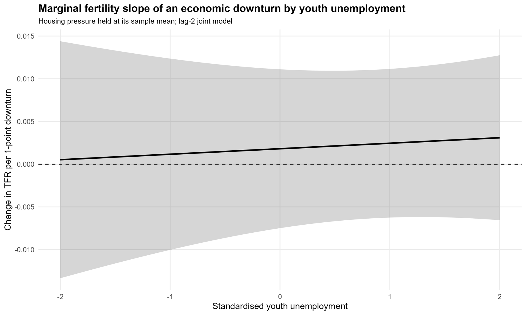
The youth-unemployment results differ. Youth unemployment has a negative direct coefficient in M2 and M5. In M5, a one-standard-deviation increase in youth unemployment is associated with a 0.063 decrease in TFR when the shock variables equal zero (b = −0.063206, p = .013). However, the downturn × youth-unemployment interaction is small and not statistically significant (b = 0.000644, p = .739). The hypothesis that youth unemployment makes downturn effects more negative is therefore not supported in the principal model.

When aggregate unemployment is entered alongside youth unemployment in M6, neither direct unemployment coefficient is significant. Youth and aggregate unemployment correlate at r = .938 and have variance inflation factors close to nine. Separate same-sample models are consequently more informative: the direct coefficients are −0.0568 (p = .031) for youth unemployment and −0.0611 (p = .017) for aggregate unemployment. Neither variable significantly moderates downturns when used as the alternative labour-market indicator.

Hypothesis assessment. H1 is not supported: the downturn main effect is not statistically significant in the principal fixed-effects sequence (M1–M5). H2a is not supported because the direct housing-pressure coefficient is not statistically significant (M2, M3, and M5). H2b is partially supported: the downturn × housing-pressure interaction is negative and significant in M3 and M5, but it is not robust to all lag and country-trend specifications. H3a is partially supported: youth unemployment has a negative direct association in M2 and M5, but joint attribution is weakened by its very high collinearity with aggregate unemployment in M6. H3b is not supported because the downturn × youth-unemployment interaction is not statistically significant in the preferred two-year-lag models (M4 and M5) and is unstable across robustness specifications.

The estimated direct and interaction coefficients from the principal fixed-effects specifications are illustrated in Figure 1.

Figure 1. Key direct and interaction coefficients from the principal fixed-effects models.

Figure 1 highlights the contrast between the statistically significant housing interaction and the null youth-unemployment interaction. It also shows that the estimated direct youth-unemployment association is larger than the interaction terms.

4.3 Marginal Effects and Substantive Magnitude

The interaction coefficient is statistically significant, but its substantive size is small. At average housing and youth unemployment, a five-percentage-point downturn is associated with an estimated TFR change of 0.0091 (95% CI [−0.0374, 0.0555]). At housing pressure one standard deviation above the mean and average youth unemployment, the corresponding change is −0.0086 (95% CI [−0.0562, 0.0390]), equal to approximately −0.55% of mean TFR. At high housing and high youth unemployment, the estimated change is −0.0054 (95% CI [−0.0479, 0.0371]). Each conditional downturn effect has a confidence interval that includes zero.

Figure 2 illustrates how the estimated marginal effect of an economic downturn varies across different levels of standardised housing pressure.

Figure 2. Estimated downturn slope across standardised housing pressure in M5.

The estimated downturn slope becomes more negative as housing pressure rises, which is the pattern captured by the significant interaction. The uncertainty band, however, underscores that the conditional downturn slope at any particular housing level is imprecisely estimated.

Figure 3 illustrates how the estimated marginal effect of an economic downturn on fertility varies across different levels of standardised youth unemployment, holding housing pressure at its sample mean.

Figure 3. Estimated downturn slope across standardised youth unemployment in M5.

The estimated fertility effects of a five-percentage-point economic downturn under alternative housing-pressure and youth-unemployment conditions are presented in Table 5.

Table 5. Substantive effects of a five-percentage-point downturn under selected moderator values.

Scenario	Δ TFR	95% CI	% of mean TFR	p
Average housing and youth unemployment	0.0091	[-0.0374, 0.0555]	0.58%	= .703
High housing, average youth unemployment	-0.0086	[-0.0562, 0.0390]	-0.55%	= .722
High housing, high youth unemployment	-0.0054	[-0.0479, 0.0371]	-0.34%	= .803
Low housing, low youth unemployment	0.0235	[-0.0329, 0.0799]	1.49%	= .414
Note. Low and high moderator values are −1 and +1 standard deviation. Effects combine the downturn main effect and all relevant interaction terms.

4.4 Regional Heterogeneity

The Southern-Europe test does not support a stronger housing-conditioned downturn effect in that region. The difference between Southern Europe and all other regions is 0.0112 (p = .071), and the difference between Southern and Western Europe is 0.0016 (p = .840). The estimated Southern European slope is −0.0008 (p = .521).

The four-region model yields a negative slope for Eastern Europe (−0.0372, p = .004) and a marginally negative slope for Northern Europe (−0.0127, p = .073), but the regional estimates are exploratory. The Eastern estimate is based on six countries and 105 observations, and multiple regional contrasts increase the risk of chance findings. The study therefore does not reframe regional heterogeneity as a central result.

The region-specific estimates of the downturn × housing-pressure interaction are presented in Figure 4.

Figure 4. Region-specific estimates of the downturn × housing-pressure slope.

4.5 Robustness and Estimator Comparisons

The housing interaction is robust to several, but not all, alternatives. It remains negative and significant with first differences (b = −0.0045, p < .001), regional interactions (b = −0.0037, p = .012), education moderation (b = −0.0040, p = .024), and dynamic fixed effects (b = −0.0043, p < .001). It is not significant with a one-year lag (p = .800), an average lag of years t−1 and t−2 (p = .523), or country-specific linear trends (p = .149). The timing sensitivity directly limits claims of universal robustness.

The youth interaction is less stable and changes sign across specifications: it is negative under the one-year lag, positive in first differences and the dynamic fixed-effects model, and null under the principal lag, average-lag, and country-trend specifications. This instability confirms that the evidence does not support a consistent moderating role for youth unemployment. The sensitivity of the principal downturn interaction coefficients to alternative model specifications is summarised in Table 6.

Table 6. Selected robustness estimates for the downturn interactions.

Specification	Downturn × housing	p	Downturn × youth unemployment	p
One-year lag	0.0003	= .800	-0.0040	= .036
Average of lags 1–2	-0.0015	= .523	-0.0038	= .296
First differences	-0.0045	< .001	0.0071	< .001
Country-specific trends	-0.0013	= .149	-0.0001	= .951
Regional interactions	-0.0037	= .012	-0.0010	= .681
Education moderation	-0.0040	= .024	0.0008	= .672
Dynamic fixed effects	-0.0043	< .001	0.0054	< .001
Note. The dynamic fixed-effects specification is a sensitivity analysis rather than a preferred causal estimator.

The downturn × housing coefficient in M5 remains significant using country-clustered standard errors (p = .012), two-way country-and-year clustering (p < .001), and Driscoll–Kraay standard errors (p = .024). The corresponding FE, RE, and Mundlak coefficients are nearly identical, although the tests disagree about the strict random-effects restrictions. These results support coefficient stability across estimators, but do not eliminate concerns about endogeneity or non-stationarity. A detailed comparison of the key coefficients across the fixed-effects, random-effects, and Mundlak specifications is presented in Table A2 in the Appendix.

4.6 Family-Policy Controls

Family-policy controls are estimated on reduced samples with paired same-sample baselines. The policy samples range from 436 to 553 country-year observations and from 30 to 36 countries. Table 7A reports the key downturn interactions before and after each policy control is added on exactly the same observations; Table 7B reports the policy coefficients themselves. Public family/children expenditure, public childcare expenditure, family allowances, and total in-kind family benefits are not statistically significant. Formal childcare participation under age three has a small negative coefficient at the 10% level (b = −0.00236, p = .063), which should not be interpreted as evidence that childcare reduces fertility because the measure is aggregate, the design is non-causal, and countries with low fertility may expand services in response to demographic conditions. Parental-leave expenditure has a positive coefficient in the single-control model (b = 0.2519, p = .015) and in the combined model (b = 0.2532, p = .044). Overall, the reduced-sample family-policy specifications yield mixed results. The paired baselines show that part of the coefficient variation reflects sample composition, while additional changes occur after particular policy controls are introduced. These models therefore neither uniformly confirm nor uniformly overturn the principal findings and should be interpreted as non-causal sensitivity analyses.

Table 7A. Same-sample comparison of key interactions before and after adding family-policy controls.

Policy model	N(countries)	D × H: baseline → + policy	D × U: baseline → + policy
P1 Family/children expenditure	553 (36)	−0.0032 (.031) → −0.0031 (.036)	−0.0002 (.894) → −0.0001 (.962)
P2 Formal childcare	534 (36)	−0.0044 (.005) → −0.0038 (.004)	0.0006 (.739) → −0.0002 (.913)
P3 Maternity/parental leave	466 (30)	−0.0024 (.253) → −0.0009 (.655)	−0.0030 (.147) → −0.0042 (.045)
P4 Public childcare expenditure	466 (30)	−0.0024 (.253) → −0.0023 (.265)	−0.0030 (.147) → −0.0031 (.168)
P5 Family allowances	466 (30)	−0.0024 (.253) → −0.0026 (.196)	−0.0030 (.147) → −0.0025 (.226)
P6 In-kind family expenditure	466 (30)	−0.0024 (.253) → −0.0024 (.255)	−0.0030 (.147) → −0.0030 (.155)
P7 Combined controls	436 (30)	−0.0030 (.189) → −0.0010 (.595)	−0.0034 (.086) → −0.0053 (.003)
Note. Cells report coefficients with p values in parentheses. D × H denotes Downturn × Housing Pressure; D × U denotes Downturn × Youth Unemployment. Baseline and augmented models use exactly the same observations. N is the number of country-year observations; countries are shown in parentheses.

Table 7B. Family-policy coefficients in same-sample augmented models.

Model	Policy set	Policy term	b	SE	p
P1	Family/children expenditure	family children expenditure gdp	0.0259	0.0400	= .522
P2	Formal childcare	formal childcare under 3	-0.0024	0.0012	= .063
P3	Maternity/parental-leave expenditure	parental leave spending gdp	0.2519	0.0974	= .015
P4	Public childcare expenditure	childcare spending gdp	0.0562	0.1308	= .671
P5	Family allowances	cash family benefits gdp	0.0642	0.0744	= .396
P6	Total in-kind family expenditure	in kind family benefits gdp	-0.0025	0.1185	= .983
P7	Combined family-policy controls	family children expenditure gdp	0.0054	0.0576	= .926
P7	Combined family-policy controls	formal childcare under 3	-0.0018	0.0013	= .176
P7	Combined family-policy controls	parental leave spending gdp	0.2532	0.1205	= .044
Note. Policy coefficients are associational robustness controls. Sample sizes and paired baseline/augmented interaction comparisons are reported in Table 7A.

5 Discussion

The analysis produces a more qualified account of economic conditions and fertility than the original specification. First, downturns do not have a statistically detectable uniform association with TFR. This is consistent with the view that macroeconomic contractions pass through institutions, household resources, employment positions, and expectations rather than generating a mechanically identical demographic response across Europe (Comolli, 2017; Sobotka et al., 2011).

Second, housing pressure is associated with the way fertility responds to downturns. The negative interaction is present in the preferred two-year-lag model, after aggregate-unemployment adjustment, with alternative standard errors, and in several robustness specifications. The result supports the idea that affordability constraints can amplify the demographic relevance of adverse macroeconomic conditions. It also aligns with recent individual-level evidence that the fertility implications of housing-market change differ sharply between renters, prospective buyers, and established owners (van Wijk, 2024; van Wijk & Feijten, 2025).

The result should not be overstated. The implied TFR changes are small, conditional slopes have wide confidence intervals, and the interaction is not significant in the one-year-lag, average-lag, or country-trend models. The evidence is therefore best described as a recurring conditional association rather than a large or universally robust causal effect. The country-trend sensitivity is especially important because TFR and several controls are persistent, and some panel unit-root tests do not reject non-stationarity.

Third, youth unemployment is more clearly associated with fertility directly than as a moderator. Its direct coefficient is negative when youth unemployment is entered without aggregate unemployment, and aggregate unemployment produces a similarly negative coefficient in a parallel same-sample model. Neither indicator consistently changes the downturn slope. The youth series covers ages 15–24, so it may capture delayed labour-market integration and household independence more than unemployment at the typical age of childbirth. The results therefore support the relevance of labour-market insecurity, but do not establish that it magnifies cyclical downturn effects.

Fourth, the regional analysis does not support the proposition that the housing-conditioned downturn slope is stronger in Southern Europe. The Southern estimate is close to zero, and the contrast with Western Europe is not significant. The negative Eastern European estimate is exploratory and based on only six countries. This finding is substantively useful because it prevents the housing-regime theory from being converted into an assumed empirical ranking. Regional institutions may still shape fertility through tenure, home-leaving, family transfers, and policy design, but the particular triple interaction tested here does not isolate a stronger Southern effect.

The reduced-sample family-policy models provide mixed rather than uniform robustness evidence. Parental-leave expenditure is positively associated with TFR in reduced samples, but the data do not support causal interpretation. Some changes in the housing and youth-interaction coefficients are already visible in the paired baselines, whereas others emerge after policy controls are added. Policy provision may be endogenous to demographic trends; expenditure measures do not capture eligibility, replacement rates, duration, service quality, or distribution; and policy data reduce the country-year sample. The paired-baseline design clarifies whether changes arise from the control itself, or from sample composition, but the restricted coverage prevents strong conclusions.

5.1 Limitations

The study uses aggregate country-year data and cannot identify individual fertility transitions, parity, partnership status, tenure, income, or subjective uncertainty. The results are vulnerable to ecological interpretation and should not be translated into individual causal effects. TFR is a period measure that responds to the timing of births, as well as completed family size, so a downturn-associated change may represent postponement, rather than a permanent reduction in cohort fertility.

The housing-overburden series restricts the main analysis to 2005–2024 and 36 countries, and all principal conditional coefficients are identified from this common analytical sample. Youth unemployment covers ages 15–24 and is not a perfect match for the age range of most first and subsequent births. Housing overburden is a population-wide measure, rather than a measure for young adults or prospective parents.

Unobserved time-varying confounding, reverse causality in policy variables, and measurement differences across countries remain possible. Fixed effects remove time-invariant heterogeneity, but do not by themselves establish causality. Serial correlation, cross-sectional dependence, and persistent series complicate inference. Alternative covariance estimators, first differences, country trends, RE/Mundlak models, and the dynamic fixed-effects specification reduce reliance on one model, but the sensitivity of some results is in itself evidence for caution.

The analysis estimates multiple interactions and robustness specifications. The regional and policy results are therefore treated as secondary evidence rather than independent discoveries. Future research should combine this macro-panel design with EU-SILC, register, or longitudinal microdata; examine age-specific and parity-specific fertility; distinguish renters, owners, and co-resident young adults; and test whether the relevant housing and labour-market exposures are concentrated among the populations actually at risk of childbearing.

6 Policy Implications

The findings do not imply that a single housing subsidy will generate a large fertility response. They indicate that housing affordability forms part of the environment in which economic shocks are translated into family decisions. Policies with the strongest theoretical connection to the mechanism include expanding the supply of affordable and family-sized dwellings, improving rental security, reducing abrupt housing-cost burdens, and lowering barriers to residential independence. Such policies may reduce postponement constraints even when their immediate effect on aggregate TFR is modest.

Youth labour-market policies remain relevant because youth and aggregate unemployment have negative direct associations with TFR when assessed separately. Stable entry jobs, predictable contracts, training-to-employment pathways, and income protection may support the establishment of the economic prerequisites of parenthood. The null moderation result means, however, that these policies should not be justified by claiming that youth unemployment demonstrably amplifies every downturn.

Family policy is most plausibly effective as a coherent package rather than as isolated short-term incentives. Paid leave with adequate replacement, accessible childcare, and financial support can reduce the incompatibility between employment and parenthood (OECD, 2024). The positive parental-leave expenditure coefficient in the robustness models is compatible with this view, but it is not causal evidence. Conversely, the marginal negative childcare coefficient is not evidence against childcare provision; it likely reflects aggregate policy endogeneity and cross-national composition.

Experience with explicit pronatalist transfers and housing-linked programmes reinforces the need for restraint. CSOK ties housing grants and subsidised credit to existing or promised children, whereas Russia’s Maternity Capital can be used for housing improvements or mortgage costs, children’s education or childcare, or the mother’s pension. These designs may relax genuine housing and liquidity constraints, but they also concentrate benefits among eligible households and can affect birth timing or selected parity transitions more readily than completed fertility. Evidence from Poland’s Family 500+ programme, Hungary’s housing-linked instruments, and Russia’s maternity-capital programmes remains mixed and heterogeneous (Bokun, 2024; Proshin, 2023; Sági & Lentner, 2022; Slonimczyk & Yurko, 2014; Vakulenko et al., 2023). Policy should therefore focus on durable constraints and family well-being, rather than on numerical birth targets alone.

7 Conclusion

This study examined whether European TFR responds differently to economic expansions and downturns, whether housing pressure and unemployment are directly associated with fertility, and whether they moderate the response to macroeconomic shocks. The analysis explicitly applied the same interaction design to housing pressure and youth unemployment, and used two-year lags as the principal specification.

The evidence does not support a broad direct effect of downturns. Housing pressure is associated with a more negative downturn–fertility slope in the preferred models, but the implied TFR changes are small and the interaction is sensitive to some timing and trend alternatives. Youth unemployment has a negative direct association when assessed without aggregate unemployment, but it does not consistently moderate downturn effects. Aggregate unemployment produces a similar direct association and likewise does not operate as a stable moderator.

The most defensible conclusion is therefore conditional and limited: affordability constraints appear to shape how adverse economic conditions relate to fertility, but the estimated demographic magnitude is modest and cannot be treated as a definitive causal effect. Policies that improve housing affordability, employment security, and work–family compatibility may reduce barriers to family formation, yet the results do not justify expectations of a large fertility rebound from any single intervention.

Acknowledgments

The authors would like to thank the editors and anonymous reviewers for their valuable comments and suggestions, which contributed to improving the clarity and quality of the manuscript.

Data availability statement

All underlying data are publicly available from the World Bank World Development Indicators, Eurostat, and the OECD Social Expenditure Database. The analysis code constructs the panel, estimates the models, and exports the tables and figures used in this manuscript. The reproducibility package can be supplied with the revised submission or deposited in a public repository, subject to the journal’s procedures.

Ethics Approval

Ethics approval was not required for this study, as the research was based exclusively on publicly available, aggregated country-level secondary data obtained from the World Bank, Eurostat, and OECD databases. No human participants were recruited, and no identifiable personal data were collected or processed.

Coauthor contributions

Anastasios D. Statiou: Data curation, investigation, writing – original draft, writing – review and editing

Peter Hatzopoulos: Conceptualization, validation, visualization

References

1. Adsera, A. (2004). Changing fertility rates in developed countries: The impact of labor market institutions. Journal of Population Economics, 17(1), 17-43. https://doi.org/10.1007/s00148-003-0166-x
2. Adsera, A. (2005). Vanishing children: From high unemployment to low fertility in developed countries. American Economic Review, 95(2), 189-193. https://doi.org/10.1257/000282805774669763
3. Adsera, A. (2011). The interplay of employment uncertainty and education in explaining second births in Europe. Demographic Research, 25, 513-544. https://doi.org/10.4054/DemRes.2011.25.16
4. Alderotti, G., Vignoli, D., Baccini, M., & Matysiak, A. (2021). Employment instability and fertility in Europe: A meta-analysis. Demography, 58(3), 871-900. https://doi.org/10.1215/00703370-9164737
5. Andersson, G. (2000). The impact of labour-force participation on childbearing behaviour: Pro-cyclical fertility in Sweden during the 1980s and the 1990s. European Journal of Population, 16(4), 293-333. https://doi.org/10.1023/A:1006454909642
6. Becker, G. S. (1960). An economic analysis of fertility. In National Bureau of Economic Research (Ed.), Demographic and economic change in developed countries (pp. 209-240). Princeton University Press.
7. Becker, G. S. (1991). A treatise on the family (Enlarged ed.). Harvard University Press.
8. Becker, G. S., & Lewis, H. G. (1973). On the interaction between the quantity and quality of children. Journal of Political Economy, 81(2, Part 2), S279-S288. https://doi.org/10.1086/260166
9. Bignami, S., Endrich, M., Natale, F., & Ueffing, P. (2024). Low fertility in the EU: A review of trends and drivers (JRC137492). Publications Office of the European Union. https://publications.jrc.ec.europa.eu/repository/handle/JRC137492
10. Bokun, A. (2024). Cash transfers and fertility: Evidence from Poland’s Family 500+ policy. Demographic Research, 51, 855-910. https://doi.org/10.4054/DemRes.2024.51.28
11. Castles, F. G., & Ferrera, M. (1996). Home ownership and the welfare state: Is Southern Europe different?. South European Society and Politics, 1(2), 163-185. https://doi.org/10.1080/13608749608539470
12. Comolli, C. L. (2017). The fertility response to the Great Recession in Europe and the United States: Structural economic conditions and perceived economic uncertainty. Demographic Research, 36, 1549-1600. https://doi.org/10.4054/DemRes.2017.36.51
13. Currie, J., & Schwandt, H. (2014). Short- and long-term effects of unemployment on fertility. Proceedings of the National Academy of Sciences, 111(41), 14734-14739. https://doi.org/10.1073/pnas.1408975111
14. Dettling, L. J., & Kearney, M. S. (2014). House prices and birth rates: The impact of the real estate market on the decision to have a baby. Journal of Public Economics, 110, 82-100. https://doi.org/10.1016/j.jpubeco.2013.09.009
15. Easterlin, R. A. (1975). An economic framework for fertility analysis. Studies in Family Planning, 6(3), 54-63. https://doi.org/10.2307/1964934
16. Eurostat. (2026). EU fertility rate at 1.34 live births per woman in 2024. European Commission. https://ec.europa.eu/eurostat/web/products-eurostat-news/w/ddn-20260306-1
17. Gauthier, A. H. (2007). The impact of family policies on fertility in industrialized countries: A review of the literature. Population Research and Policy Review, 26(3), 323-346. https://doi.org/10.1007/s11113-007-9033-x
18. Gil-Solsona, D. (2023). ‘Not really leaving home’ in Southern Europe: Intermediate living situations in Catalan youth housing trajectories. Journal of Youth Studies, 26(8), 1084-1107. https://doi.org/10.1080/13676261.2022.2065912
19. Goldstein, J. R., Sobotka, T., & Jasilioniene, A. (2009). The end of “lowest-low” fertility?. Population and Development Review, 35(4), 663-699. https://doi.org/10.1111/j.1728-4457.2009.00304.x
20. Kalwij, A. (2010). The impact of family policy expenditure on fertility in Western Europe. Demography, 47(2), 503-519. https://doi.org/10.1353/dem.0.0104
21. Kreyenfeld, M. (2010). Uncertainties in female employment careers and the postponement of parenthood in Germany. European Sociological Review, 26(3), 351-366. https://doi.org/10.1093/esr/jcp026
22. Kulu, H., & Steele, F. (2013). Interrelationships between childbearing and housing transitions in the family life course. Demography, 50(5), 1687-1714. https://doi.org/10.1007/s13524-013-0216-2
23. Luppi, F., Rosina, A., & Sironi, E. (2024). Leaving and returning to the parental home during COVID times in France, Italy, Germany, Spain, and the United Kingdom. Demographic Research, 50, 101-114. https://doi.org/10.4054/DemRes.2024.50.3
24. Matysiak, A., & Vignoli, D. (2024). Family life courses, uncertain futures, and the changing world of work: State-of-the-art and prospects. European Journal of Population, 40(1), 19. https://doi.org/10.1007/s10680-024-09701-x
25. Mulder, C. H. (2006). Home-ownership and family formation. Journal of Housing and the Built Environment, 21(3), 281-298. https://doi.org/10.1007/s10901-006-9050-9
26. Mulder, C. H., & Billari, F. C. (2010). Homeownership regimes and low fertility. Housing Studies, 25(4), 527-541. https://doi.org/10.1080/02673031003711469
27. Neyer, G., & Andersson, G. (2008). Consequences of family policies on childbearing behavior: Effects or artifacts?. Population and Development Review, 34(4), 699-724. https://doi.org/10.1111/j.1728-4457.2008.00246.x
28. OECD. (2024). Society at a glance 2024: OECD social indicators. OECD Publishing. https://doi.org/10.1787/918d8db3-en
29. Proshin, A. (2023). Impact of child subsidies on child health, well-being, and investment in child human capital: Evidence from Russian Longitudinal Monitoring Survey 2010-2017. European Journal of Population, 39(1), 14. https://doi.org/10.1007/s10680-023-09653-8
30. Schneider, D. (2015). The Great Recession, fertility, and uncertainty: Evidence from the United States. Journal of Marriage and Family, 77(5), 1144-1156. https://doi.org/10.1111/jomf.12212
31. Schwanitz, K., Rampazzo, F., & Vitali, A. (2021). Unpacking intentions to leave the parental home in Europe using the Generations and Gender Survey. Demographic Research, 45, 17-54. https://doi.org/10.4054/DemRes.2021.45.2
32. Slonimczyk, F., & Yurko, A. (2014). Assessing the impact of the maternity capital policy in Russia. Labour Economics, 30, 265-281. https://doi.org/10.1016/j.labeco.2014.03.004
33. Sobotka, T., Skirbekk, V., & Philipov, D. (2011). Economic recession and fertility in the developed world. Population and Development Review, 37(2), 267-306. https://doi.org/10.1111/j.1728-4457.2011.00411.x
34. Sági, J., & Lentner, C. (2022). Key issues in the effectiveness of public financial tools to support childbearing: The example of Hungary during the COVID-19 crisis. PLOS ONE, 17(8), e0273090. https://doi.org/10.1371/journal.pone.0273090
35. Vakulenko, E. S., Ivashina, N. V., & Svistyilnik, Y. O. (2023). Regional maternity capital programmes: Impact on fertility in Russia. Economy of Regions, 19(4), 1077-1092. https://doi.org/10.17059/ekon.reg.2023-4-10
36. van Wijk, D. (2024). House prices and fertility: Can the Dutch housing crisis explain the post-2010 fertility decline?. Population, Space and Place, 30(7). https://doi.org/10.1002/psp.2787
37. van Wijk, D., & Billari, F. C. (2024). Fertility postponement, economic uncertainty, and the increasing income prerequisites of parenthood. Population and Development Review, 50(2), 287-322. https://doi.org/10.1111/padr.12624
38. van Wijk, D., & Feijten, P. (2025). Rising house prices, falling fertility? How rising house prices widen fertility differences between tenure groups. European Journal of Population, 41(1), 33. https://doi.org/10.1007/s10680-025-09754-6

Country Coverage

Table A1. List of the 36 European countries contributing at least one observation to the principal common two-year-lag sample.

Region	Country	ISO3	Main N
Western Europe	Austria	AUT	10
Western Europe	Belgium	BEL	19
Western Europe	France	FRA	18
Western Europe	Germany	DEU	10
Western Europe	Luxembourg	LUX	13
Western Europe	Netherlands	NLD	14
Western Europe	Switzerland	CHE	14
Eastern Europe	Bulgaria	BGR	17
Eastern Europe	Czechia	CZE	18
Eastern Europe	Hungary	HUN	18
Eastern Europe	Poland	POL	18
Eastern Europe	Romania	ROU	16
Eastern Europe	Slovak Republic	SVK	18
Northern Europe	Denmark	DNK	18
Northern Europe	Estonia	EST	18
Northern Europe	Finland	FIN	19
Northern Europe	Iceland	ISL	17
Northern Europe	Ireland	IRL	20
Northern Europe	Latvia	LVA	18
Northern Europe	Lithuania	LTU	18
Northern Europe	Norway	NOR	19
Northern Europe	Sweden	SWE	19
Northern Europe	United Kingdom	GBR	14
Southern Europe	Albania	ALB	6
Southern Europe	Croatia	HRV	13
Southern Europe	Cyprus	CYP	18
Southern Europe	Greece	GRC	16
Southern Europe	Italy	ITA	19
Southern Europe	Malta	MLT	18
Southern Europe	Montenegro	MNE	10
Southern Europe	North Macedonia	MKD	10
Southern Europe	Portugal	PRT	8
Southern Europe	Serbia	SRB	10
Southern Europe	Slovenia	SVN	18
Southern Europe	Spain	ESP	19
Southern Europe	Turkiye	TUR	17
Note. Main N is the number of country-year observations contributed by each country to the common two-year-lag estimation sample.

Additional estimator comparison

Table A2. Comparison of the key coefficients under fixed effects, conventional random effects, and the full Mundlak correlated-random-effects model.

term	FE full interaction	RE full interaction	Mundlak CRE full interaction
boom_l2	0.0034 (0.0049)	0.0032 (0.0047)	0.0034 (0.0050)
downturn_l2	0.0018 (0.0047)	0.0016 (0.0042)	0.0019 (0.0047)
z_housing_l2	-0.0052 (0.0285)	-0.0019 (0.0238)	-0.0054 (0.0290)
z_youth_l2	-0.0632*** (0.0239)	-0.0652*** (0.0185)	-0.0631*** (0.0242)
boom_housing_l2	-0.0023 (0.0022)	-0.0023 (0.0024)	-0.0022 (0.0023)
downturn_housing_l2	-0.0035*** (0.0013)	-0.0035** (0.0015)	-0.0035*** (0.0013)
boom_youth_l2	0.0021 (0.0030)	0.0023 (0.0031)	0.0022 (0.0030)
downturn_youth_l2	0.0006 (0.0019)	0.0008 (0.0021)	0.0006 (0.0019)
log_gdp_pc_l2	0.0150 (0.2736)	-0.0060 (0.0717)	0.0212 (0.2769)
female_lfp_l2	0.0031 (0.0087)	0.0027 (0.0060)	0.0031 (0.0089)
tertiary_female_l2	-0.0014 (0.0015)	-0.0012 (0.0014)	-0.0013 (0.0015)
Note: The interaction coefficients are similar across estimators; the Mundlak joint test nevertheless rejects the restriction that all country means are zero.

Data codes and selections

To preserve reproducibility while keeping the main variable table concise, the source codes and dataset selections removed from Table 1 are reported here.

Table A3. Source codes and dataset selections.

Variable	Code / selection
Total fertility rate (TFR)	SP.DYN.TFRT.IN
GDP per capita	NY.GDP.PCAP.KD
Real GDP-per-capita growth	NY.GDP.PCAP.KD
Economic expansion	Derived
Economic downturn	Derived
Housing-cost overburden rate	ilc_lvho07a; unit=PC; rskpovth=TOTAL; age=TOTAL; sex=T
Youth unemployment rate	SL.UEM.1524.ZS
Aggregate unemployment rate	SL.UEM.TOTL.ZS
Female labour-force participation	SL.TLF.CACT.FE.ZS
Female tertiary gross enrolment	SE.TER.ENRR.FE
Family/children social-protection expenditure	spr_exp_func; spdeps=SPR; spfunc=FAM; unit=PC_GDP
Formal childcare participation under the age of three	tepsr_sp210; age=Y_LT3; duration=H_GE1; unit=PC
Maternity and parental-leave expenditure	unit=PT_B1GQ; programme=TP512; spending=C
Public childcare expenditure	unit=PT_B1GQ; programme=TP521; spending=K
Family-allowance expenditure	unit=PT_B1GQ; programme=TP511; spending=C
Total in-kind family expenditure	unit=PT_B1GQ; programme=TP51; spending=K
Annual house-price growth	prc_hpi_a; purchase=TOTAL; unit=RCH_A_AVG
Note. Codes and selections reproduce the source identifiers used to construct the analytical variables.